Posts

Successfully graphed both test targets and graphed the PCA waterband depth plot

Image
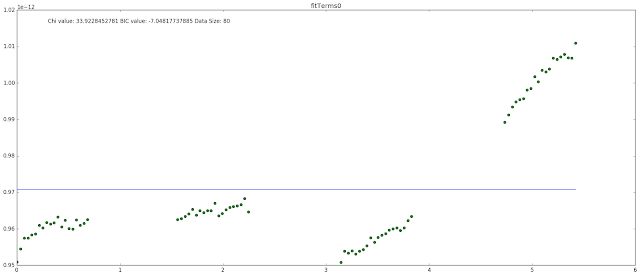
I have successfully moved forward with several things on my to do list. First off I have successfully graphed both test targets after reducing them. I extracted them with an extraction width of 7. We can change this to match the Apai paper. I did this by copying one of the regular star location images, since the code wanted at least 2 star location images. The code then ran perfectly fine after reduction on all the test target data. I have also taken Dylan's PCA code, modified it somewhat, and have used it successfully to graph a waterband depth plot for the 2 test targets and the 2 targets I'm working on. I just used an array of 1's to calculate the error since I have not learned how to calculate the error for a pca plot. The test data does not perfectly match our data, but that is most likely because the parameters used to extract the data using aXe are not exactly the same, as well as the systematic errors are not accounted for in the test data. However the variation

working on the waterband graphs

Image
Today I found something interesting playing around with the test data. I found that when graphing just the raw data, I got a very noisy looking graph with only a sort of dip in the waterband. I thought this was strange, especially since in the paper they have a very clear dip in the waterband. Through some experimenting I found that using a rolling mean to smooth out the data, I produced nearly the exact same graph as was produced in the paper, with the same type of features in the waterband. I then did this same thing on the data that we have and produced a much cleaner and clear signal than what we had before. I included the test data and the data we are currently working with as well. The smoothing I think brings out a better waterband feature for both test targets that we have been working with. SIMP0136 2MASS-J16291840 SDSS-J075

Working on Latex as well as fixed graph bumpiness

Image
Today I have been working on a few different items. I have attempted to start a latex paper for what we are going to be working on, but have been unable to get emulateapj to work. I will continue to work on it until it is solved. I believe I have conflicting installation of Tex and there is a bad directory somewhere which is causing emulateapj to not be seen.  However I solved the problem of the bumpy curve fit by removing two uneccesary parameters (which was probably the cause of the bumpiness). The smooth curve fit is shown below. The two pictures shown below have very similar BIC values, with three being just a tiny bit lower. However 4 has a lower chi value which is a much better fit. The target shown is 2MASS-J16291840+0335371

waterband depth and graphing variables seperatly

Image
Today I worked on producing a waterband depth graph, which turned out to be more complex than I first thought, especially when propagating the error through to the end. I have left an example of one of the waterband depth plots at the bottom of this post. I've also been working on graphing the variables separately for the curve_fit function, which I did successfully. Interestingly enough, each sin cosine pair came out smooth. However, when fit for the function as a whole, the graph comes out bumpy. I also asked the internet about any ideas of what it could be, and I got the answer that it was an expected behavior of the curve_fit function. I've also included pictures below.

flux percentage graphs

Image
Today I've been working on several different items. First I have figured out why the flux percentage was failing. I was summing the edges of the data and that for whatever reason was causing the whole flux to drop significantly. By only summing the flux from 10600 to 17000 I found that it greatly stabilized the result and I got exactly what I was expected to get. I added to the upper left when less than a percent changes. It is pictured below. Interestingly enough, I found that the extraction width is fairly close to the optimal noise for the waterband. This can show that using the noise in the waterband as a guide to choosing an extraction width agrees with using the amount of total flux captured.
Image
These are several different fits, each one gaining another pair of variables in the fourier transformation. The fit is about the same from 4 parameters on and actually gets worse when getting to large numbers of parameters. I've also included the chi value and the BIC value on every single graph. The BIC value as of right now increases fairly linearly as I add more parameters. Here are some additional graphs I've been working on that have been fit with a fourier fit of 4 different terms 2MASS-J16291840+0335371 SDSS-J075840.33+324723.4

Current Graphs

Image
SDSS-J075840.33+324723.4 2MASS-J16291840+0335371 (first set of exposures) 2MASS-J16291840+0335371 (second set of exposures)